Comparing two datasets with Venn Diagram

Cordeliers Artificial Intelligence and Bioinformatics

2025-06-23

Here is an example of an application for the function plot_venn. For this script, we used 2 different public datasets airway and macrophage.

If you want to use this notebook for your projects, it is available here

The airway dataset provides a gene expression dataset derived from human bronchial epithelial cells, treated or not with dexamethasone (a corticosteroid).

The macrophage dataset provides bulk RNA-seq count data from human monocyte-derived macrophages. These cells were either left untreated or stimulated with interferon-gamma (IFN-γ).
An experimental condition was applied to each of these cells, left unstimulated, stimulated with IFN-gamma, infected with SL1344, or pre-treated with IFN-g and then infected with SL1344. For this comparison, we will focus on the samples of the 2 first conditions (IFN-g, naive).

To compare the datasets, we will do the pre-processing part of the sup and unsup analysis, until the diffexp.

annotation_air <- "dex"
annotation_mac <- "condition_name"

diffexpMethod <- "limma"

Import libraries

library(airway)
library(SummarizedExperiment)
library(macrophage)
library(biomaRt)
library(CAIBIrnaseq)

Load datasets

#Loading the 2 datasets
data(airway, package="airway"); 
airway <- airway

data("gse")
macrophage <- gse; rm(gse)
macrophage <- macrophage[,macrophage$condition %in% c("naive", "IFNg")] # focus on these 2 conditions

Even if the datasets are globally build the same way, the names of the variables are not exactly the same, so if we want to keep the same code, we need to redefine a bit the variables.

If you want to know what are the used variables in this part, run this command line : colnames(SummarizedExperiment::rowData(exp_data))

You should have these variables (with these exact same names):
- gene_name : The commonly used symbol or name for the gene (e.g., A1BG).
- gene_id : A unique and stable identifier for the gene, often from databases like Ensembl (e.g., ENSG00000141510).
- gene_length_kb : The length of the gene measured in kilobases
- gene_description : A brief textual summary of the gene’s function or characteristics, often pulled from annotation databases.
- gene_biotype : A classification of the gene based on its biological function or transcript type, such as protein_coding, lncRNA, or pseudogene.

If not, you should look at how your dataset is defined. You might need to run some command line as the following ones:

rowData(airway)$gene_length_kb <-(rowData(airway)$gene_seq_end - rowData(airway)$gene_seq_start) / 1000

mart_air <- useEnsembl("ensembl", dataset = "hsapiens_gene_ensembl")

gene_ids_air <- rowData(airway)$gene_id

annot_air <- getBM(attributes = c("ensembl_gene_id", "description"),
               filters = "ensembl_gene_id",
               values = gene_ids_air,
               mart = mart_air)

matched_air <- match(rowData(airway)$gene_id, annot_air$ensembl_gene_id)
rowData(airway)$gene_description <- annot_air$description[matched_air]

rowData(macrophage)$gene_length_kb <- width(rowRanges(macrophage)) / 1000
rownames(macrophage) <- sub("\\..*$", "", rowData(macrophage)$gene_id)
rowData(macrophage)$gene_id <- sub("\\..*$", "", rowData(macrophage)$gene_id)

rowData(macrophage)$gene_name <- rowData(macrophage)$SYMBOL

macrophage <- macrophage[!is.na(rowData(macrophage)$SYMBOL), ]

mart_mac <- useEnsembl("ensembl", dataset = "hsapiens_gene_ensembl")

annot_mac <- getBM(
  attributes = c("ensembl_gene_id", "gene_biotype", "description"),
  filters = "ensembl_gene_id",
  values = unique(rowData(macrophage)$gene_id),
  mart = mart_mac
)
# Correspondance entre gene_id et annot_mac
match_mac <- match(rowData(macrophage)$gene_id, annot_mac$ensembl_gene_id)

# Ajouter les colonnes dans rowData
rowData(macrophage)$gene_biotype <- annot_mac$gene_biotype[match_mac]
rowData(macrophage)$gene_description <- annot_mac$description[match_mac]

Pre-processing

Most datasets use ensembl gene ID by default after alignment, so this step rebases the expression data to gene names. This ensures consistency in naming for downstream analyses.

airway <- rebase_gexp(airway, annotation = "gene_name")

macrophage <- rebase_gexp(macrophage, annotation = "SYMBOL") # or gene_name if you renamed the variable 

Filter

Here, we filter out genes expressed in too few samples or with very low counts. This removes noise from the data and focuses on meaningful gene expressions.

airway <- filter_gexp(airway,
                        min_nsamp = 1, 
                        min_counts = 1)

macrophage <- filter_gexp(macrophage,
                        min_nsamp = 1, 
                        min_counts = 1)

Quality Control

Visualization of the filtering process to ensure the criteria applied align with the dataset’s characteristics:

colData(airway)$sample_id <- colnames(airway)
plot_qc_filters(airway)

colData(macrophage)$sample_id <- colnames(macrophage)
plot_qc_filters(macrophage)

Normalize

Here, we apply a normalization to the expression data, making samples comparable by reducing variability due to technical differences. For datasets with few samples, rlog is the preferred normalization and when more samples are present, vst is applied.

airway <- normalize_gexp(airway)
assay(macrophage) <- round(assay(macrophage))
macrophage <- normalize_gexp(macrophage)

PCA

Principal component analysis (PCA) identifies the major patterns in the dataset. These patterns help explore similarities or differences among samples based on gene expression.

#|message: false
metadata(airway)[["pca_res"]] <- pca_gexp(airway)
annotations <- setdiff(annotation_air, c("exp_cluster", "path_cluster"))
plot_pca(airway, color = annotation_air)

metadata(macrophage)[["pca_res"]] <- pca_gexp(macrophage)
annotations <- setdiff(annotation_mac, c("exp_cluster", "path_cluster"))
plot_pca(macrophage, color = annotation_mac)

Diffexp

Differential expression analysis is a key step in RNA-seq data interpretation. It aims to identify genes whose expression levels significantly change between experimental conditions—in this case, between treated and untreated airway samples, and between IFNg-stimulated and naive macrophages. By statistically testing gene expression differences, this analysis highlights biologically relevant genes that may be involved in specific cellular responses or disease mechanisms. .

library(edgeR)
colData(airway)$dex <- factor(colData(airway)$dex)
colData(airway)$dex <- factor(colData(airway)$dex, levels = c("untrt", "trt")) #  change with your conditions' names


diffexp_air <- diffExpAnalysis(countData = assays(airway)$counts,
                                          sampleInfo = colData(airway),
                                          method = diffexpMethod, cutoff = 10,
                                          annotation = annotation_air)

colData(macrophage)$condition_name <- factor(colData(macrophage)$condition_name)
colData(macrophage)$condition_name <- factor(colData(macrophage)$condition_name, levels = c("IFNg", "naive"))


diffexp_mac <- diffExpAnalysis(countData = assays(macrophage)$counts,
                                          sampleInfo = colData(macrophage),
                                          method = diffexpMethod, cutoff = 10,
                                          annotation = annotation_mac)

Venn Diagram

Once the diffexp done, we can plot the venn diagram. Since the datasets are not directly related, it could be interesting to see if there are still similarities. The comparison can be made between genes, pathways, …

If there are similarities, it can means that some biological processes are activated for different condition types.

This diagram show us how much genes are unique to one dataset, and which are in common. The fisher test value corresponds to the reliability of this analysis. The nearer it is to 0, the most significant this analysis is.

#|message: false
if(tolower(diffexpMethod) == "limma") {     # you can change it with 'DESeq2'
  diffexp_air <- diffexp_air |>
    dplyr::rename(
      log2FoldChange = logFC,
      pvalue = P.Value,
      padj = adj.P.Val
    )
}

if(tolower(diffexpMethod) == "limma"){
  diffexp_mac <- diffexp_mac |>
    dplyr::rename(
      log2FoldChange = logFC,
      pvalue = P.Value,
      padj = adj.P.Val
    )
}

# Exemple : extraction des degs_airgènes DE significatifs
degs_air <- rownames(diffexp_air[diffexp_air$padj < 0.05, ])    # you can change the threshold 'padj'
degs_mac <- rownames(diffexp_mac[diffexp_mac$padj < 0.05, ])
# universe_size <- length(union(degs_air, degs_mac))
universe_size <- 7000

# Diagramme de Venn
plot_venn(degs_air, degs_mac, universe_size,
          v1_name = "Airway", v2_name = "Macrophage",
          fills = c("lightgreen", "skyblue"),
          title = "DEGs communs et spécifiques")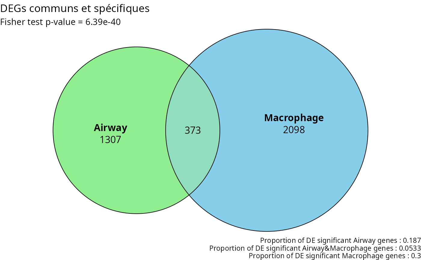

trt <- airway[,colData(airway)$dex == "trt"]

Additional analyses

Collections

The airway and macrophage datasets have some common genes. We can visualize it with the venn diagram. Now that we know that, maybe we can further analyse whether it is ‘random’ or something about a biological process.

inter <- intersect(degs_air, degs_mac)

msigdbr::msigdbr_collections() |>
  kableExtra::kbl() |>
  kableExtra::kable_styling() |>
  kableExtra::scroll_box(height = "300px")

gs_collection	gs_subcollection	gs_collection_name	num_genesets
C1		Positional	302
C2	CGP	Chemical and Genetic Perturbations	3494
C2	CP	Canonical Pathways	19
C2	CP:BIOCARTA	BioCarta Pathways	292
C2	CP:KEGG_LEGACY	KEGG Legacy Pathways	186
C2	CP:KEGG_MEDICUS	KEGG Medicus Pathways	658
C2	CP:PID	PID Pathways	196
C2	CP:REACTOME	Reactome Pathways	1736
C2	CP:WIKIPATHWAYS	WikiPathways	830
C3	MIR:MIRDB	miRDB	2377
C3	MIR:MIR_LEGACY	MIR_Legacy	221
C3	TFT:GTRD	GTRD	505
C3	TFT:TFT_LEGACY	TFT_Legacy	610
C4	3CA	Curated Cancer Cell Atlas gene sets	148
C4	CGN	Cancer Gene Neighborhoods	427
C4	CM	Cancer Modules	431
C5	GO:BP	GO Biological Process	7608
C5	GO:CC	GO Cellular Component	1026
C5	GO:MF	GO Molecular Function	1820
C5	HPO	Human Phenotype Ontology	5653
C6		Oncogenic Signature	189
C7	IMMUNESIGDB	ImmuneSigDB	4872
C7	VAX	HIPC Vaccine Response	347
C8		Cell Type Signature	840
H		Hallmark	50

Volcano

The 2 volcano plots show us top 15 differential expressed genes.

#|message: false
diffexp_air$gene <- rownames(diffexp_air)
diffexp_mac$gene <- rownames(diffexp_mac)

# Gènes significatifs (par exemple padj < 0.05)
sig_air <- diffexp_air[diffexp_air$padj < 0.05, ]
sig_mac <- diffexp_mac[diffexp_mac$padj < 0.05, ]

# Gènes en commun (par nom de gène)
common_genes <- intersect(sig_air$gene, sig_mac$gene)

# Sous-ensemble des jeux avec uniquement les gènes communs
common_air <- diffexp_air[diffexp_air$gene %in% common_genes, ]
common_mac <- diffexp_mac[diffexp_mac$gene %in% common_genes, ]

plot_exp_volcano(common_air, 15)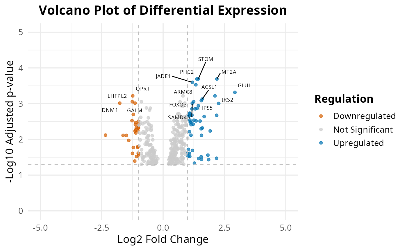

plot_exp_volcano(common_mac, 15)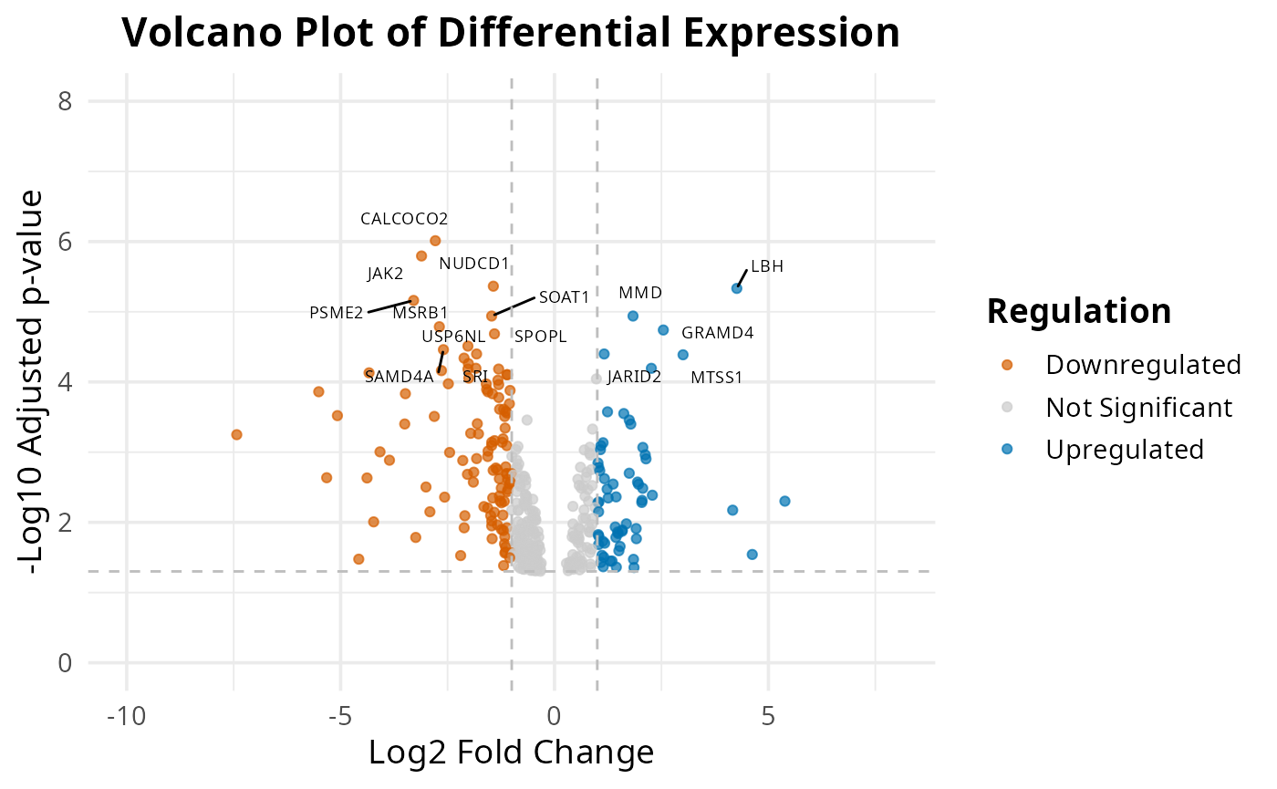

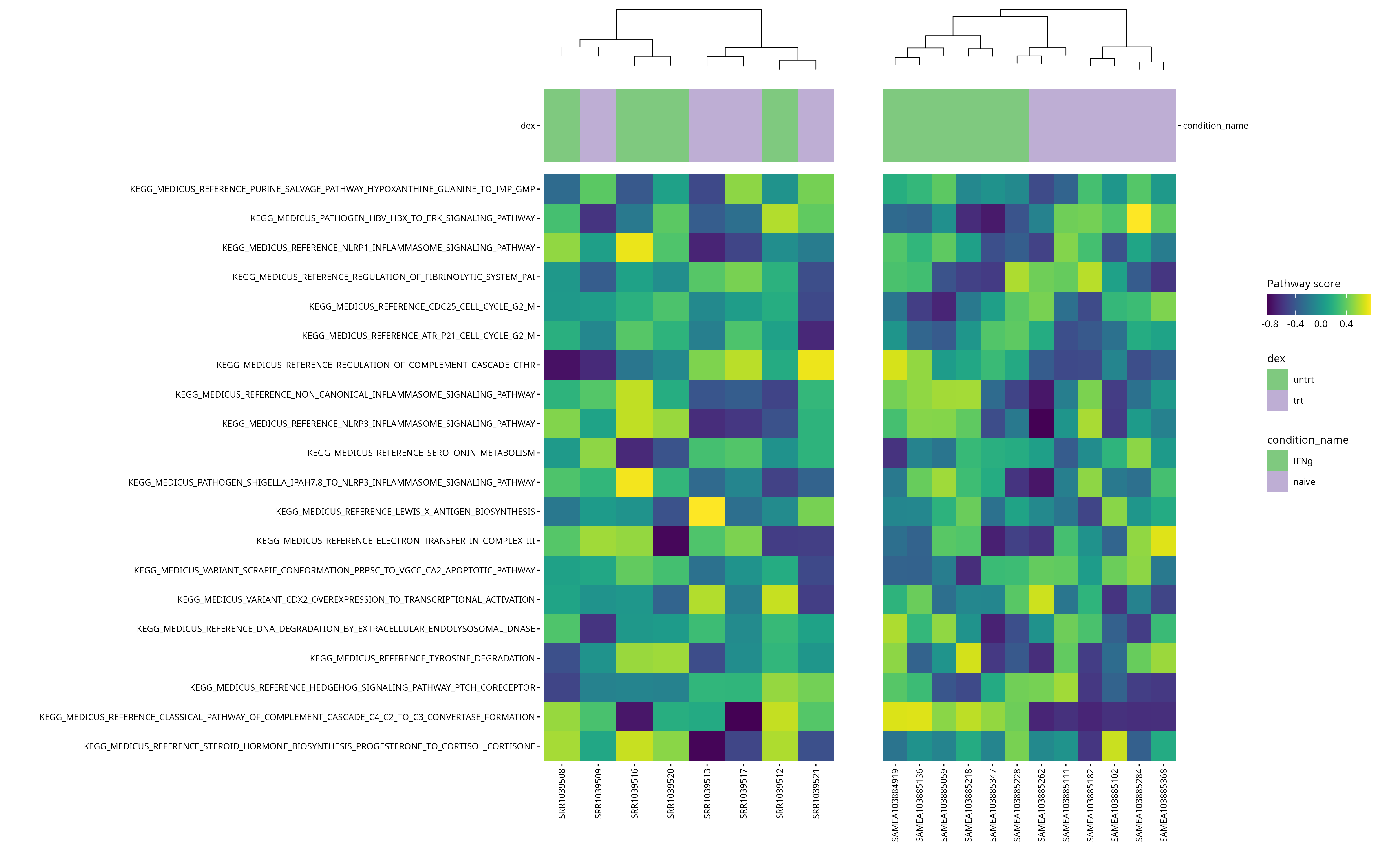
Heatmaps

dir.create("results", "airway", "pathways")
dir.create("results", "macrophage", "pathways")


pathway_collections <- c("CP:KEGG_MEDICUS")

pathways <- get_annotation_collection(pathway_collections, 
                                      species = "human")
scores_airway <- score_pathways(airway, pathways, verbose = FALSE)
scores_macrophage <- score_pathways(macrophage, pathways, verbose = FALSE)

# Identifier les pathways communs
common_paths <- intersect(rownames(scores_airway), rownames(scores_macrophage))## Warning in prep_scores_hm(exp_data, progeny_scores): 'sample_id' already exists

# Définir un ordre commun basé sur les scores moyens dans airway
order_common <- rowMeans(scores_airway[common_paths, , drop = FALSE]) |>
  sort(decreasing = TRUE) |>
  names()

# Re-générer les heatmaps dans le même ordre
collections <- pathway_collections |> 
  paste(collapse = "_") |> 
  stringr::str_remove("\\:")

# Réordonner les matrices selon cet ordre
scores_airway <- scores_airway[order_common, ]
scores_macrophage <- scores_macrophage[order_common, ]

# Remplacer les anciennes matrices dans les objets
metadata(airway)[["pathway_scores"]] <- scores_airway
metadata(macrophage)[["pathway_scores"]] <- scores_macrophage

dir.create("results", "airway", "pathways")
dir.create("results", "macrophage", "pathways")


# airway
plt_air <- plot_pathway_heatmap(airway, annotations = annotation_air,
                     fwidth = 9,
                     cluster_rows = FALSE,
                     fname = stringr::str_glue("results/airway/pathways/hm_paths_{collections}_top20_aligned.pdf"))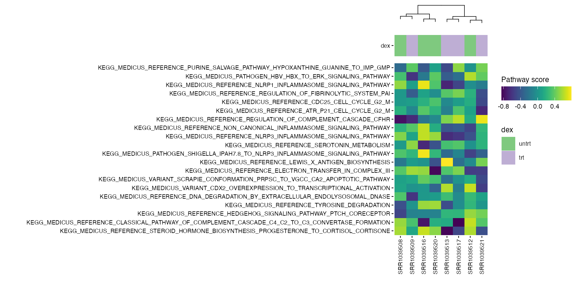

# macrophage
plt_mac <- plot_pathway_heatmap(macrophage, annotations = annotation_mac,
                     fwidth = 9,
                     cluster_rows = FALSE,
                     show_rownames = FALSE,
                     fname = stringr::str_glue("results/macrophage/pathways/hm_paths_{collections}_top20_aligned.pdf"))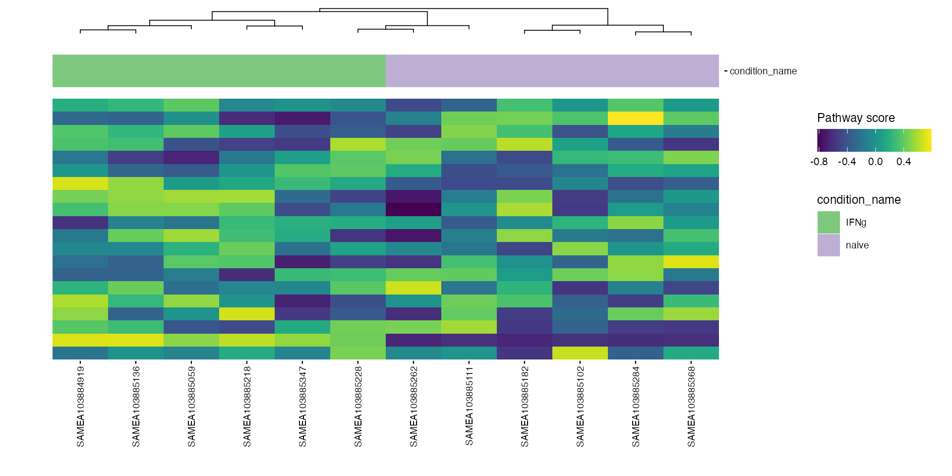

require(patchwork)
require(ggheatmapper)
ggsave("results/heatmap_big.png", align_heatmaps(plt_air, plt_mac), width = 16, height = 10, dpi = 300)

Click to zoom in :