Unsupervised RNA-seq analysis
Cordeliers Artificial Intelligence and Bioinformatics
Source:vignettes/unsup_rnaseq.Rmd
unsup_rnaseq.Rmd
As with the supervised example, we are using an open dataset which is
given by t he airway package. It provides a gene expression
dataset derived from human bronchial epithelial cells,
treated or not with dexamethasone (a
corticosteroid).
Here is an example of how the unsupervised part of
the CAIBIrnaseq package can be used.
library(airway)
library(SummarizedExperiment)
library(CAIBIrnaseq)
library(tidyverse)
Parameters
species <- "Homo sapiens"   # Or "Mus musculus"

# Annotation variable to visualize
plot_annotations <- "dex"  # Put the name of the condition (here 'dex' is treated or untreated)

# Quality parameters
qc_min_nsamp <- 2
qc_min_gene_counts <- 10

# Clustering of expression
exp_cluster <- data.frame(k = 2) #Number of cluster

# Clustering of metadata
metadata_clusters <- list(
  pathway_scores = data.frame(k = 2),
  microenv_scores = data.frame(k = 3)
)

# The following variables are those that will need to be modified depending on the analyses you want to do

# Pathway collections
pathway_collections <- c("CGP", "CP", "CP:KEGG_LEGACY", "Hallmark") #See the msigdb table and modify with the interesting collections

# Interesting genes
heatmap_genes <- list(
  gr_response_genes <- c("FKBP5", "TSC22D3", "PER1", "ZBTB16"),
  anti_inflam_genes <- c("DUSP1", "SOCS1", "MT2A")
)     # same here, replace with the genes you are interested in

heatmap_pathways <- c(
  "DUTERTRE_ESTRADIOL_RESPONSE_24HR_DN",
  "REN_ALVEOLAR_RHABDOMYOSARCOMA_DN",
  "NUYTTEN_EZH2_TARGETS_UP",
  "PASINI_SUZ12_TARGETS_DN"
) #Same

# Genes for the boxplots
boxplot_genes <- c("FKBP5", "TSC22D3")  #same

# Pathways for the boxplots
boxplot_pathways <- c(
  "KUMAMOTO_RESPONSE_TO_NUTLIN_3A_UP",
  "CASTELLANO_HRAS_TARGETS_DN"
) #same

# Corrélations entre gènes
correlation_genes <- list(
  c("FKBP5", "TSC22D3"),
  c("FKBP5", "ZBTB16")
)

# Pathways correlation
correlation_pathways <- list(
  c("DUTERTRE_ESTRADIOL_RESPONSE_24HR_DN", "REN_ALVEOLAR_RHABDOMYOSARCOMA_DN"),
  c("REN_ALVEOLAR_RHABDOMYOSARCOMA_DN", "NUYTTEN_EZH2_TARGETS_UP")
)   #same
Load data
This section loads the RNA-seq dataset for analysis. It ensures the correct input file is used, as specified in the parameters. rebase_gexp
Ensure your dataset is in a Summarized Experiment
object, because all the used functions below works with
SummarizedExperiment input.
If you want to know more about this type of object, please click here: Bioconductor
data(airway, package="airway")
exp_data <- airway

# If you are using your own dataset .RDS file), use this command line :
# exp_data <- readRDS(data_file)
Even if the datasets are globally build the same way, the names of the variables are not exactly the same, so if we want to keep the same code, we need to redefine a bit the variables.
If you want to know what are the used variables in this part, run
this command line :
colnames(SummarizedExperiment::rowData(exp_data))
You should have these variables (with these exact same names):
- gene_name : The commonly used symbol or name for the
gene (e.g., A1BG).
- gene_id : A unique and stable identifier for the
gene, often from databases like Ensembl.
- gene_length_kb : The length of the gene measured in
kilobases
- gene_description : A brief textual summary of the
gene’s function or characteristics. - gene_biotype : A
classification of the gene based on its biological function or
transcript type, such as protein_coding, lncRNA, or pseudogene.
If you are using the notebook that Clarice GROENEVELD created to convert a .xsl file into a .RDS one, you can SKIP the next cell. If not, you should look at how your dataset is defined. You might need to run some command line as the following ones:
library(biomaRt)

rowData(exp_data)$gene_length_kb <-
  (rowData(exp_data)$gene_seq_end - rowData(exp_data)$gene_seq_start) / 1000

mart <- useEnsembl("ensembl", dataset = "hsapiens_gene_ensembl")
gene_ids <- rowData(exp_data)$gene_id

annot <- getBM(attributes = c("ensembl_gene_id", "description"),
               filters = "ensembl_gene_id",
               values = gene_ids,
               mart = mart)

matched <- match(rowData(exp_data)$gene_id, annot$ensembl_gene_id)
rowData(exp_data)$gene_description <- annot$description[matched]
Pre-processing
Most datasets use ensembl gene ID by default after alignment, so this step rebases the expression data to gene names. This ensures consistency in naming for downstream analyses.
exp_data <- rebase_gexp(exp_data, keep_cols = c("gene_name", "gene_id",
                                                "gene_biotype", "gene_length_kb"))
Filter
Here, we filter out genes expressed in too few samples or with very low counts. This removes noise from the data and focuses on meaningful gene expressions.
exp_data <- filter_gexp(exp_data,
                        min_nsamp = 1,
                        min_counts = 1)
Visualization of the filtering process to ensure the criteria applied align with the dataset’s characteristics:
colData(exp_data)$sample_id <- colnames(exp_data)
plot_qc_filters(exp_data)
Normalize
Here, we apply a normalization to the expression data, making samples
comparable by reducing variability due to technical differences. For
datasets with few samples, rlog is the preferred
normalization and when more samples are present, vst is
applied.
exp_data <- normalize_gexp(exp_data)PCA
Principal component analysis (PCA) identifies the major patterns in the dataset. These patterns help explore similarities or differences among samples based on gene expression.
pca_res = pca_gexp(exp_data)
exp_data@metadata[["pca_res"]] <- pca_res
annotations <- setdiff(plot_annotations, c("exp_cluster", "path_cluster"))
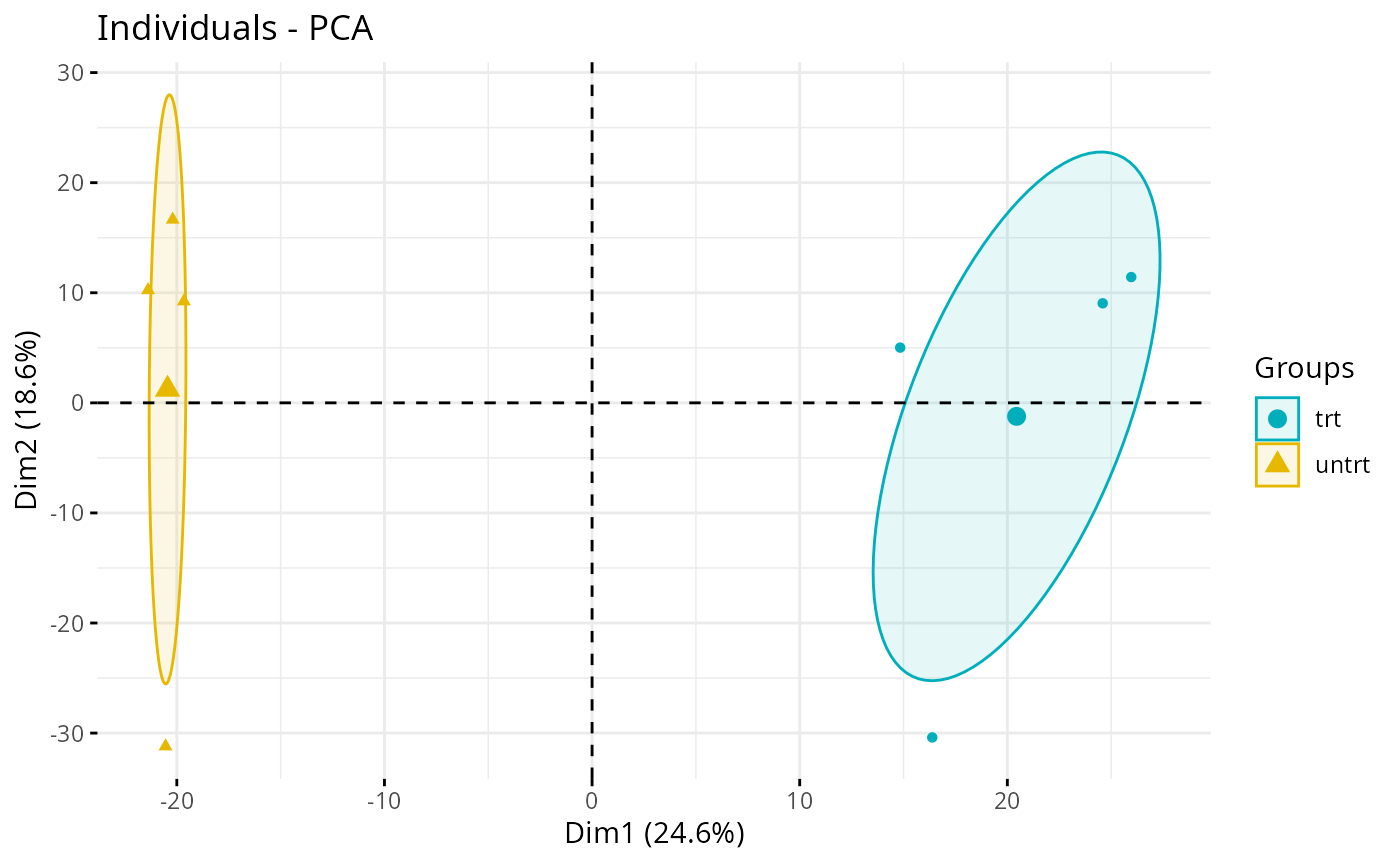
plot_pca(exp_data, color = plot_annotations)If you want something more visual, you can add a circular/oval shape
to circle the different genotypes of samples, use the
fviz_pca_ind function from the factoextra
package. With this dataset, it is not relevant but it can be with your
persona dataset. Here, it highlights the fact that the 2 groups are not
crossing each other. The trt group has more PC1, whereas
the untrt group has less. We could conclude that PC1 is
more represented in the treated samples.
library(factoextra)
groups <- SummarizedExperiment::colData(exp_data)$dex  # here we want to split in function of `treated` and `untreated`

fviz_pca_ind(pca_res,
             geom = "point",
             habillage = groups,
             palette = c("#00AFBB", "#E7B800"),  # Personalized colors
             addEllipses = TRUE,
             ellipse.type = "confidence",
             repel = TRUE,
             label = "none"
)
Unsupervised clustering
Here, we group samples based on expression patterns without prior knowledge using hierarchical clustering on either a selected gene list from the parameters or, by default, the 2000 most highly expressed genes.
This can be useful for discovering sample subgroups or new biological insights.
exp_data <- cluster_exp(exp_data, k = exp_cluster$k, genes = exp_cluster$genes, n_pcs = 3)Visual representation of expression levels for HVG across clusters, highlighting distinct patterns.
hvg <- highly_variable_genes(exp_data)
exp_cluster <- data.frame(k = 2)
hm <- plot_exp_heatmap(exp_data,  genes = hvg,
                 annotations = c(plot_annotations, "exp_cluster"),
                 show_rownames = FALSE,
                 hm_color_limits = c(-2,2),
                 fname = "results/unsup/clustering/heatmap_2000hvg_exp_cluster.pdf")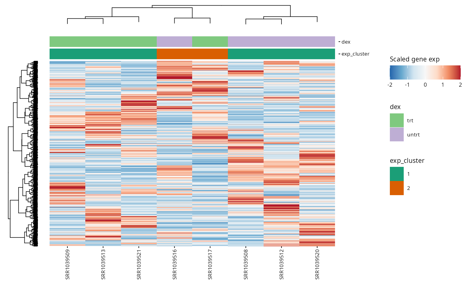
hm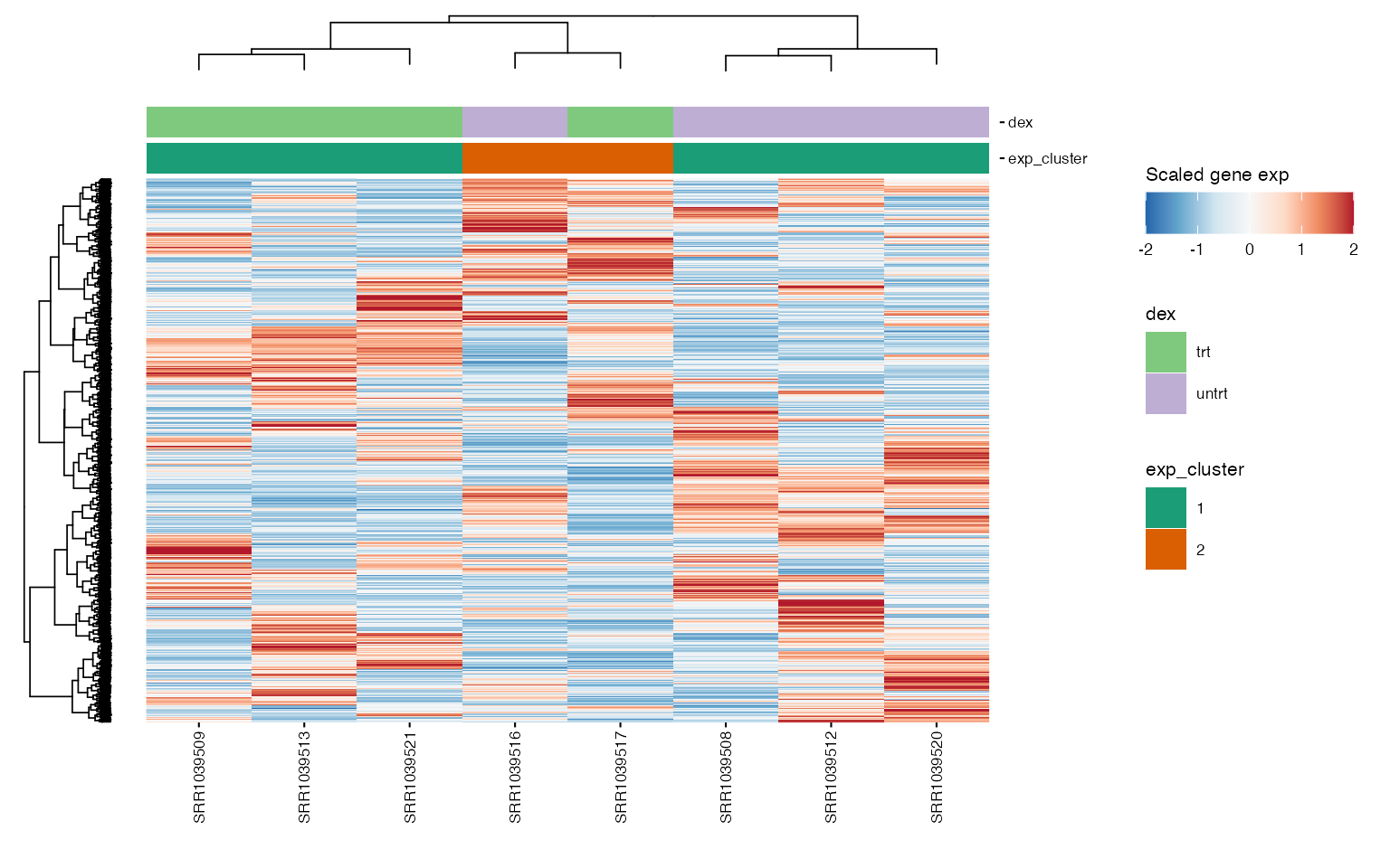
Pathway activity
Pathway analysis enables us to understand the functional implications of gene expression changes. Here, we analyze the dataset for pathway activity using two methods.
PROGENy
PROGENy is a collection of only 14 core pathway responsive genes from large signaling perturbation experiments. For more information see the original paper.
The returned plot will give us information about the pathways that
are activated for each sample. There is especially one pathway that is
highly activated : EGFR , in the sample
SRR1039517
progeny_scores <- score_progeny(exp_data, species = "Homo sapiens")
progeny_scores <- score_progeny(exp_data, species = "Homo sapiens")

metadata(exp_data)[["progeny_scores"]] <- progeny_scores

plot_progeny_heatmap(exp_data, annotations = plot_annotations,
                     fname = "results/unsup/pathways/hm_progeny_scores.pdf")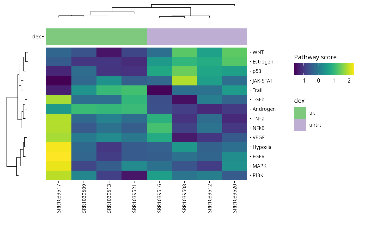

write.csv(progeny_scores, file = "results/unsup/pathways/progeny_scores.csv")Pathways
Ensure your dataset is in a Summarized Experiment
object, because all the used functions below works with
SummarizedExperiment input.
Pathway collections available in the MSIGdb can be specified in the
parameters. These pathways are scored and ranked by their variance in
the data. These are the available collections (use
gs_subcollection as name except for Hallmarks, which should
be ‘H’).
library(msigdbr)
library(dplyr)
library(kableExtra)


msigdbr::msigdbr_collections() |>
  kableExtra::kbl() |>
  kableExtra::kable_styling() |>
kableExtra::scroll_box(height = "300px")| gs_collection | gs_subcollection | gs_collection_name | num_genesets |
|---|---|---|---|
| C1 | Positional | 302 | |
| C2 | CGP | Chemical and Genetic Perturbations | 3494 |
| C2 | CP | Canonical Pathways | 19 |
| C2 | CP:BIOCARTA | BioCarta Pathways | 292 |
| C2 | CP:KEGG_LEGACY | KEGG Legacy Pathways | 186 |
| C2 | CP:KEGG_MEDICUS | KEGG Medicus Pathways | 658 |
| C2 | CP:PID | PID Pathways | 196 |
| C2 | CP:REACTOME | Reactome Pathways | 1736 |
| C2 | CP:WIKIPATHWAYS | WikiPathways | 830 |
| C3 | MIR:MIRDB | miRDB | 2377 |
| C3 | MIR:MIR_LEGACY | MIR_Legacy | 221 |
| C3 | TFT:GTRD | GTRD | 505 |
| C3 | TFT:TFT_LEGACY | TFT_Legacy | 610 |
| C4 | 3CA | Curated Cancer Cell Atlas gene sets | 148 |
| C4 | CGN | Cancer Gene Neighborhoods | 427 |
| C4 | CM | Cancer Modules | 431 |
| C5 | GO:BP | GO Biological Process | 7608 |
| C5 | GO:CC | GO Cellular Component | 1026 |
| C5 | GO:MF | GO Molecular Function | 1820 |
| C5 | HPO | Human Phenotype Ontology | 5653 |
| C6 | Oncogenic Signature | 189 | |
| C7 | IMMUNESIGDB | ImmuneSigDB | 4872 |
| C7 | VAX | HIPC Vaccine Response | 347 |
| C8 | Cell Type Signature | 840 | |
| H | Hallmark | 50 |
pathways <- get_annotation_collection(pathway_collections,
species = species)
pathway_scores <- score_pathways(exp_data, pathways, verbose = FALSE)
metadata(exp_data)[["pathway_scores"]] <- pathway_scores
collections <- pathway_collections |>
paste(collapse = "_") |>
stringr::str_remove("\\:")
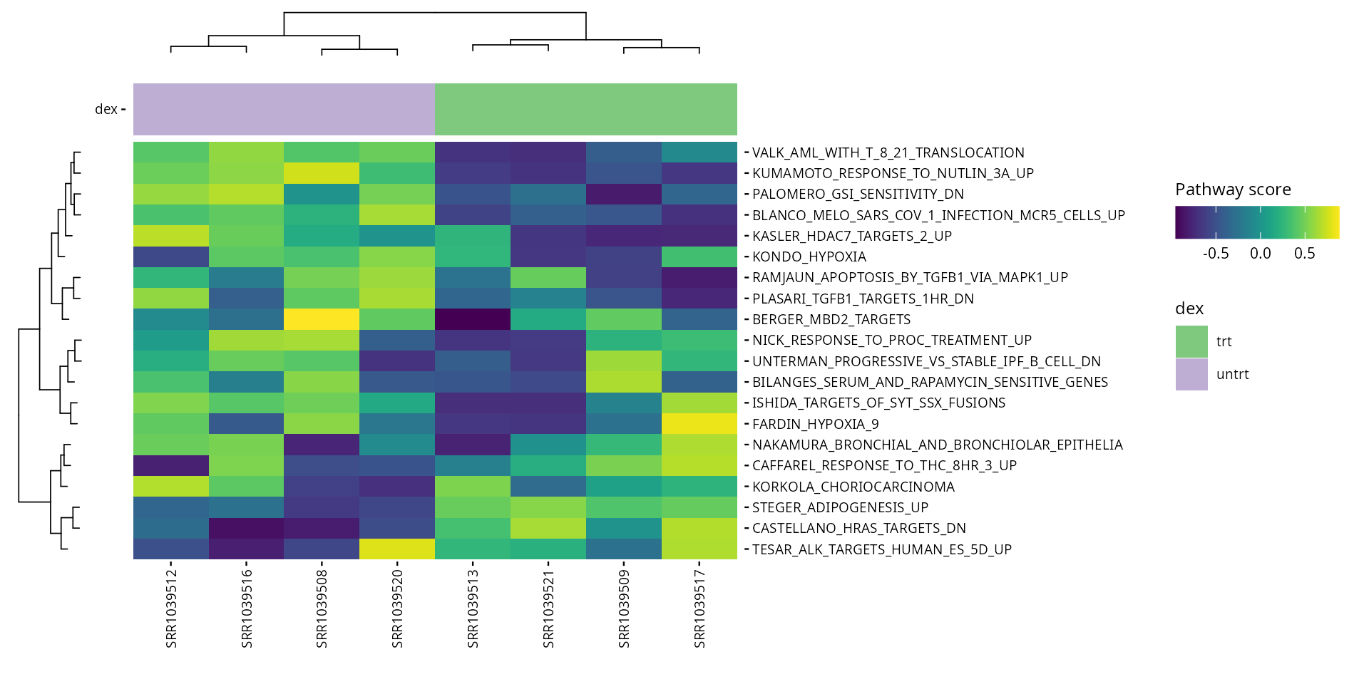
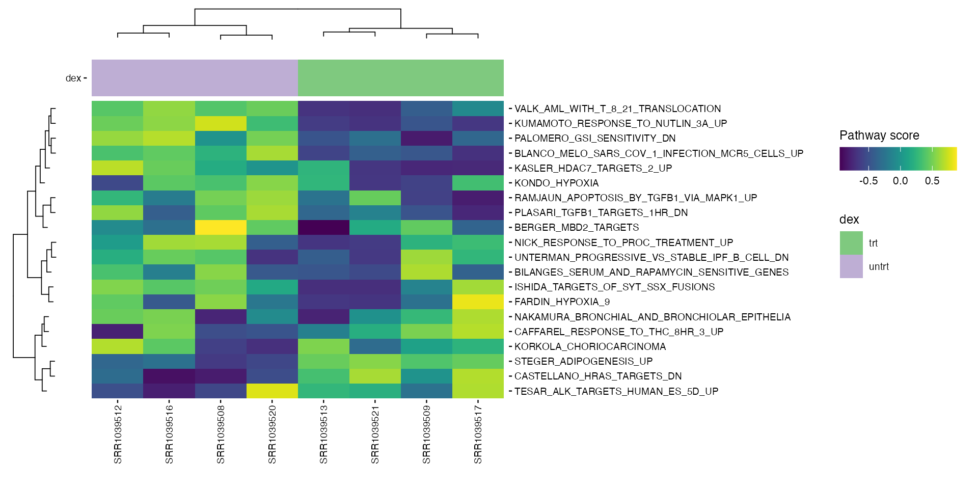
plot_pathway_heatmap(exp_data, annotations = plot_annotations,
fwidth = 9,
fname = stringr::str_glue(
"results/unsup/pathways/hm_paths_{collections}_top20.pdf")
)
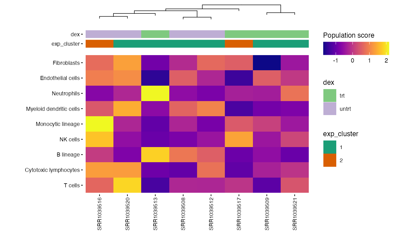
Microenvironment scores
This step calculates immune and stromal cell type abundances using MCPcounter or mMCPcounter. It helps to infer the composition of the tumor microenvironment or similar contexts.
mcp_scores <- mcp_counter(exp_data, species = species)
S4Vectors::metadata(exp_data)[["microenv_scores"]] <- mcp_scores

plot_microenv_heatmap(exp_data, annotations = c("dex", "exp_cluster"),
                      fname = "results/unsup/tme/heatSmap_mcpcounter.pdf")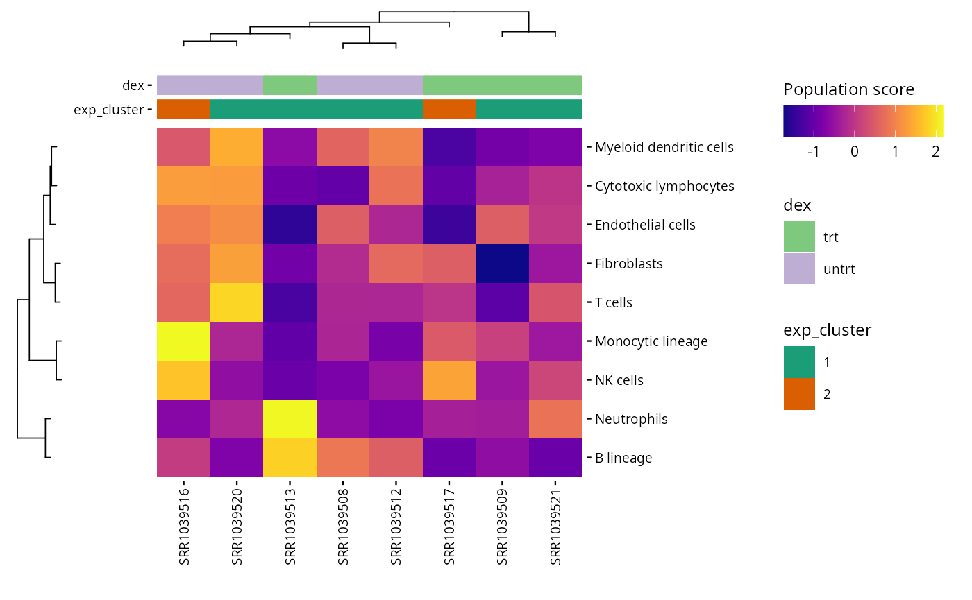
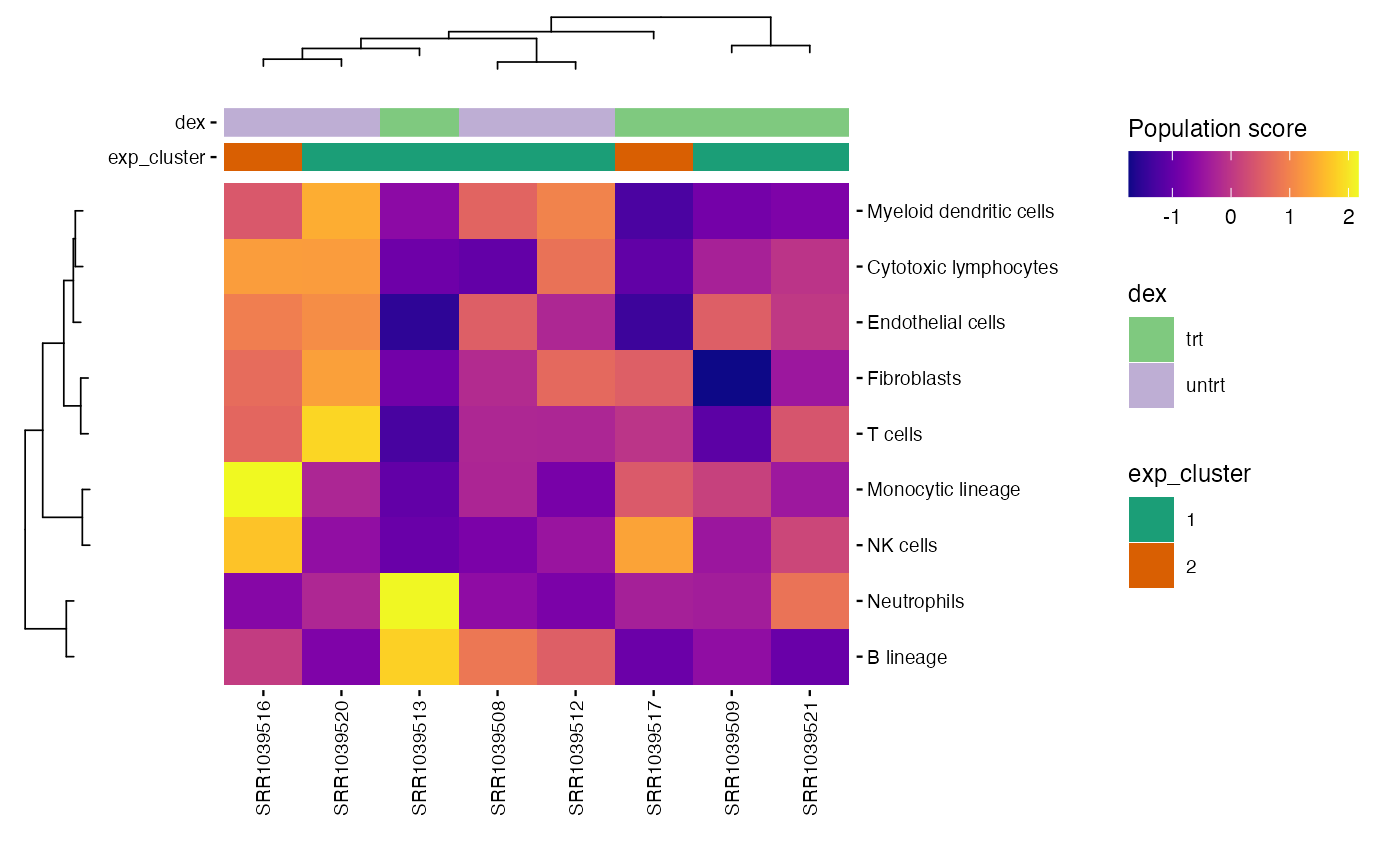
write.csv(mcp_scores, file = "results/unsup/tme/scores_mcpcounter.csv")By default, the rows are order by scores. But, the
plot_microenv_heatsmap function has the
ellipsis argument. That means that this function can have a
wide range of inputs. So, it is possible to plot the rows in a different
order than the default one :
plot_microenv_heatmap(exp_data,
                      annotations = c("dex", "exp_cluster"),
                      fname = "results/unsup/tme/heatmap_sorted_bydex.pdf",
                      cluster_rows = FALSE)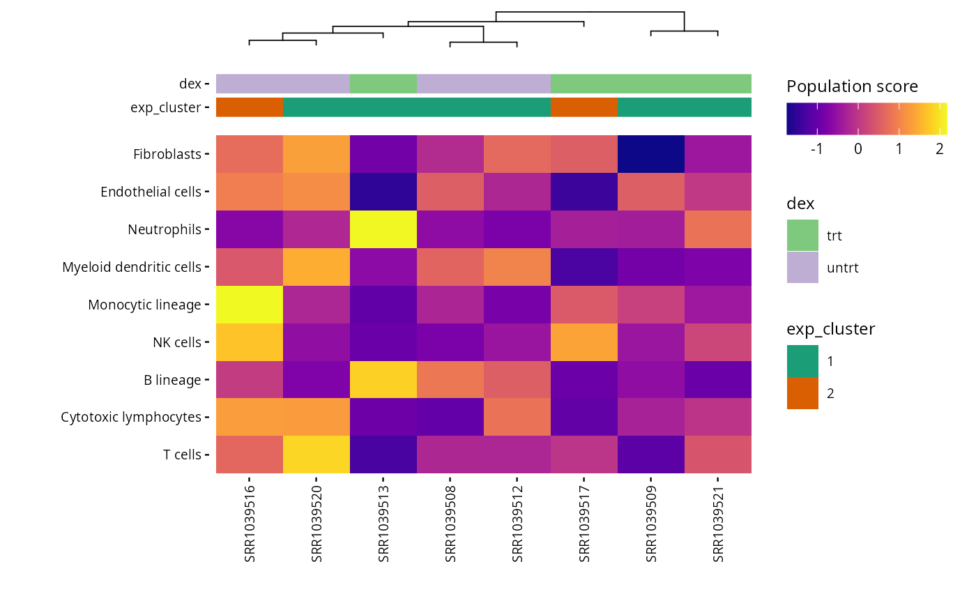
Targeted plots
This section focuses on visualizing specific genes or pathways of interest, as specified in the parameters.
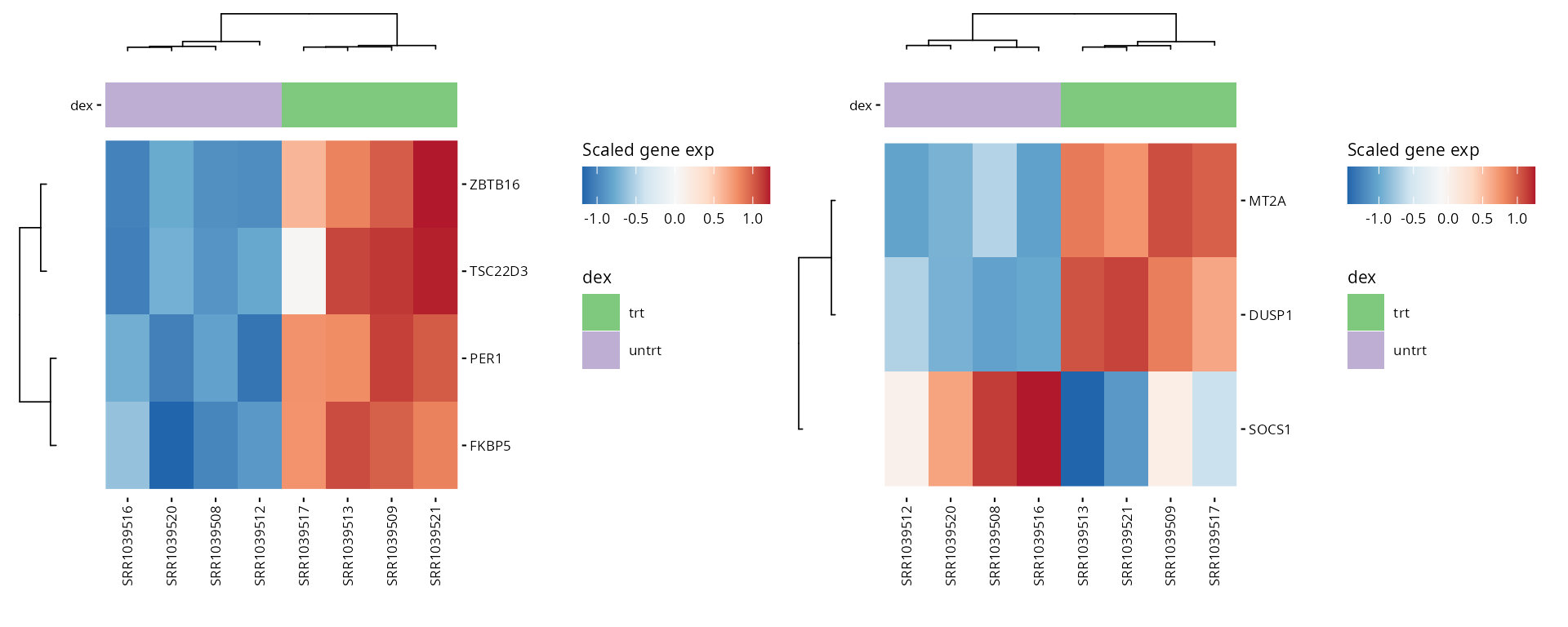
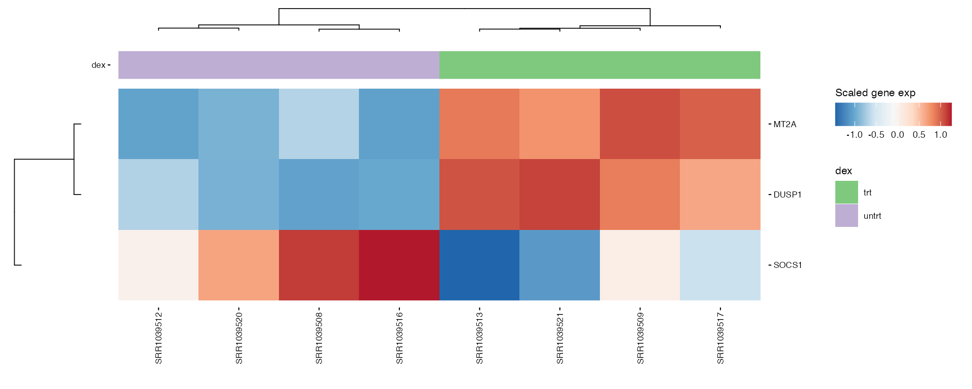
Heatmaps
Generates heatmaps for pre-selected genes of interest to observe their expression across samples or conditions.
hms <- lapply(1:length(heatmap_genes), function(i) {
  gene_annot <- SummarizedExperiment::rowData(exp_data)
  genes <- heatmap_genes[[i]]
  name <- ifelse(is.null(names(heatmap_genes)), i, names(heatmap_genes)[i])
  plot_exp_heatmap(exp_data, genes = genes,
                   annotations = plot_annotations,
                   fname = stringr::str_glue("results/unsup/targeted/hm_genes_{i}.pdf"))
})
patchwork::wrap_plots(hms, ncol = 2, guides = "collect")
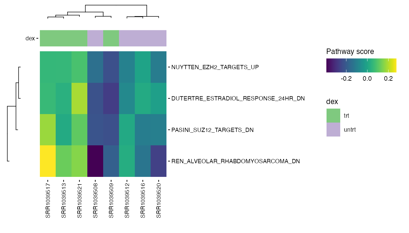
Selected pathways
valid_pathways <- intersect(heatmap_pathways, rownames(pathway_scores))

plot_pathway_heatmap(exp_data,
                     annotations = plot_annotations,
                     pathways = valid_pathways,
                     fname = stringr::str_glue("results/unsup/targeted/hm_pathways_selected.pdf"))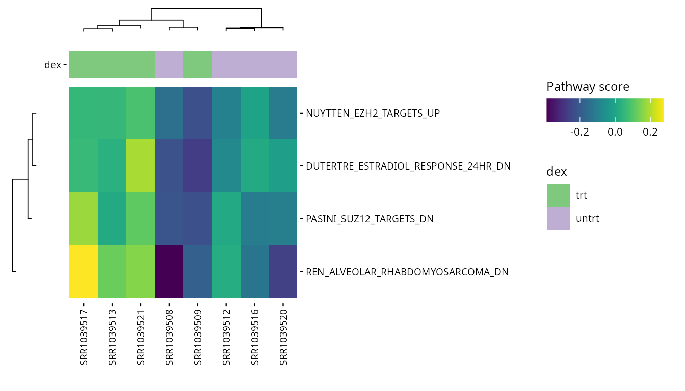
Compare clusters
Boxplots provide a clear comparison of expression levels across experimental groups or conditions.
Selected genes
genes <- boxplot_genes
annotations <- plot_annotations

boxplots <- lapply(genes, function(gene) {
  lapply(annotations, function(annotation) {
    plt <- plot_exp_boxplot(exp_data, gene = gene,
                   annotation = annotation,
                   color_var = annotation,
                   pt_size = 2,
                   fname = stringr::str_glue("results/unsup/targeted/boxplots/box_{gene}_{annotation}.pdf"))
  })
}) |> purrr::flatten()
patchwork::wrap_plots(boxplots, nrows = round(length(boxplots)/2), guides = "collect")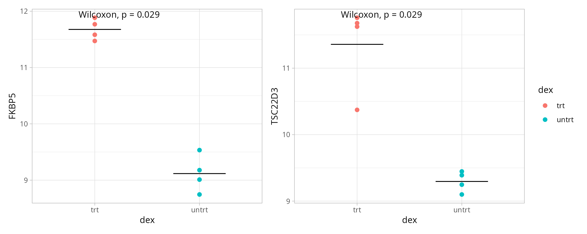
Selected pathways
paths <- boxplot_pathways
annotations <- plot_annotations

boxplots <- lapply(paths, function(path) {
  lapply(annotations, function(annotation) {
    plt <- plot_pathway_boxplot(exp_data,
                             pathway = path,
                   annotation = annotation,
                   color_var = annotation,
                   pt_size = 2,
                   fname = stringr::str_glue("results/unsup/targeted/boxplots/box_{path}_{annotation}.pdf"))
  })
}) |> purrr::flatten()
patchwork::wrap_plots(boxplots, nrows = round(length(boxplots)/2), guides = "collect")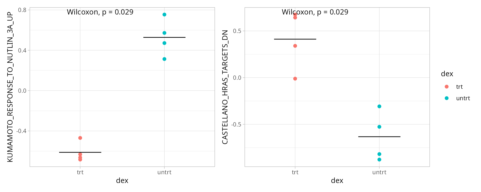
Selected pathways
Correlation plots for selected pathways can help identify similarities or differences in pathway activity patterns across samples. Each pathway pair is plotted separately and color-coded by sample annotation to illustrate trends within each condition.
path_pairs <-correlation_pathways
annotations <- plot_annotations

cor_plts <- lapply(path_pairs, function(path_pair) {
  lapply(annotations, function(annot) {
      plot_pathway_scatter(exp_data,
                   pathway1 = path_pair[1],
                   pathway2 = path_pair[2],## Call `lifecycle::last_lifecycle_warnings()` to see where this warning was
                   color_var = annot,
                   fname = stringr::str_glue(
                     "results/unsup/targeted/correlations/cor_{path_pair[1]}_{path_pair[2]}_color={annot}.pdf"))
  })
}) |> purrr::flatten()
patchwork::wrap_plots(cor_plts, nrows = round(length(cor_plts)/2), guides = "collect")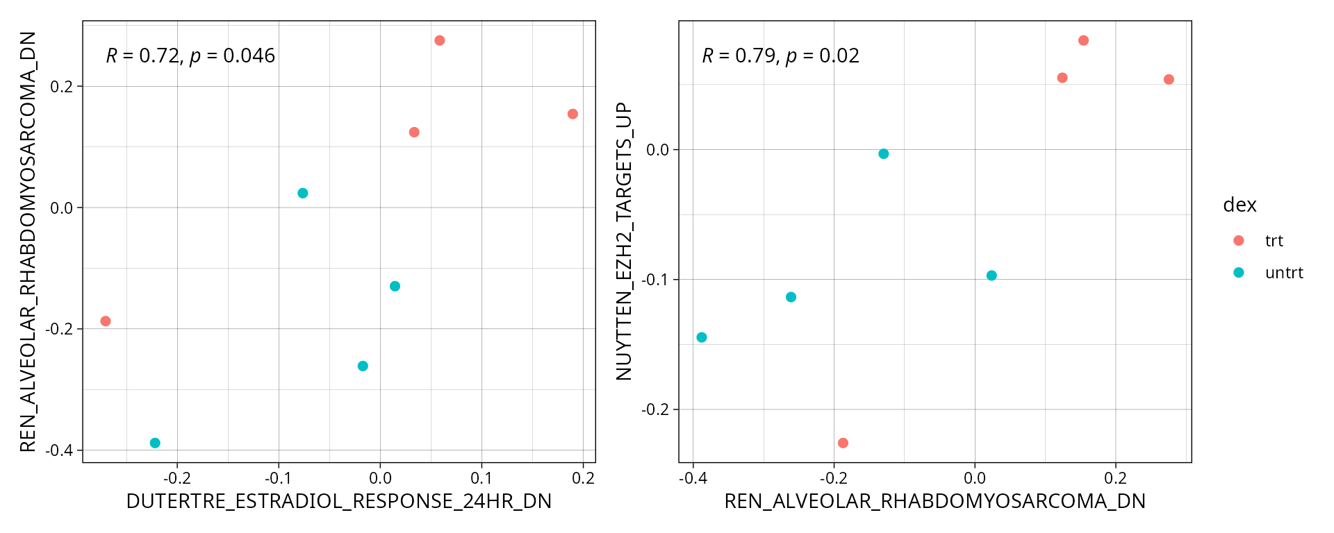
Cluster using metadata
types = names(metadata_clusters)

for(type in types) {
  exp_data <- cluster_metadata(exp_data,
                   metadata_name = type,
                   k = metadata_clusters[[type]]$k,
                   features = metadata_clusters[[type]]$features,
                   n_pcs = 3 )
}
Save SummarizedExperiment
The final step saves the processed dataset and results. This ensures all outputs can be revisited or shared for further analysis.
Report parameters
For reproducibility, the parameters used in the analysis and the computational environment details are documented.
sessionInfo
The sessionInfo() prints out all packages loaded at the
time of analysis, as well as their versions.
## R version 4.5.0 (2025-04-11)
## Platform: aarch64-apple-darwin20
## Running under: macOS Sequoia 15.5
##
## Matrix products: default
## BLAS:   /Library/Frameworks/R.framework/Versions/4.5-arm64/Resources/lib/libRblas.0.dylib
## LAPACK: /Library/Frameworks/R.framework/Versions/4.5-arm64/Resources/lib/libRlapack.dylib;  LAPACK version 3.12.1
##
## locale:
## [1] en_US.UTF-8/en_US.UTF-8/en_US.UTF-8/C/en_US.UTF-8/en_US.UTF-8
##
## time zone: Europe/Paris
## tzcode source: internal
##
## attached base packages:
## [1] stats4    stats     graphics  grDevices utils     datasets  methods
## [8] base
##
## other attached packages:
##  [1] kableExtra_1.4.0            msigdbr_10.0.2
##  [3] factoextra_1.0.7            biomaRt_2.64.0
##  [5] lubridate_1.9.4             forcats_1.0.0
##  [7] stringr_1.5.1               dplyr_1.1.4
##  [9] purrr_1.0.4                 readr_2.1.5
## [11] tidyr_1.3.1                 tibble_3.2.1
## [13] ggplot2_3.5.2               tidyverse_2.0.0
## [15] CAIBIrnaseq_1.0.1           R.utils_2.13.0
## [17] R.oo_1.27.0                 R.methodsS3_1.8.2
## [19] airway_1.28.0               SummarizedExperiment_1.38.0
## [21] Biobase_2.68.0              GenomicRanges_1.60.0
## [23] GenomeInfoDb_1.44.0         IRanges_2.42.0
## [25] S4Vectors_0.46.0            BiocGenerics_0.54.0
## [27] generics_0.1.3              MatrixGenerics_1.20.0
## [29] matrixStats_1.5.0
##
## loaded via a namespace (and not attached):
##   [1] ggplotify_0.1.2             filelock_1.0.3
##   [3] graph_1.86.0                XML_3.99-0.18
##   [5] lifecycle_1.0.4             httr2_1.1.2
##   [7] rstatix_0.7.2               lattice_0.22-7
##   [9] crosstalk_1.2.1             backports_1.5.0
##  [11] magrittr_2.0.3              plotly_4.10.4
##  [13] sass_0.4.10                 rmarkdown_2.29
##  [15] jquerylib_0.1.4             yaml_2.3.10
##  [17] rlist_0.4.6.2               RColorBrewer_1.1-3
##  [19] cowplot_1.1.3               DBI_1.2.3
##  [21] eulerr_7.0.2                abind_1.4-8
##  [23] yulab.utils_0.2.0           rappdirs_0.3.3
##  [25] GenomeInfoDbData_1.2.14     ggrepel_0.9.6
##  [27] irlba_2.3.5.1               tidytree_0.4.6
##  [29] GSVA_2.2.0                  MCPcounter_1.2.0
##  [31] annotate_1.86.0             svglite_2.1.3
##  [33] pkgdown_2.1.1               codetools_0.2-20
##  [35] DelayedArray_0.34.1         xml2_1.3.8
##  [37] tidyselect_1.2.1            aplot_0.2.5
##  [39] UCSC.utils_1.4.0            farver_2.1.2
##  [41] ScaledMatrix_1.16.0         BiocFileCache_2.16.0
##  [43] jsonlite_2.0.0              Formula_1.2-5
##  [45] systemfonts_1.2.2           tools_4.5.0
##  [47] progress_1.2.3              treeio_1.32.0
##  [49] ragg_1.4.0                  Rcpp_1.0.14
##  [51] glue_1.8.0                  gridExtra_2.3
##  [53] SparseArray_1.8.0           xfun_0.52
##  [55] DESeq2_1.48.0               HDF5Array_1.36.0
##  [57] withr_3.0.2                 fastmap_1.2.0
##  [59] rhdf5filters_1.20.0         digest_0.6.37
##  [61] rsvd_1.0.5                  timechange_0.3.0
##  [63] R6_2.6.1                    gridGraphics_0.5-1
##  [65] textshaping_1.0.0           colorspace_2.1-1
##  [67] RSQLite_2.3.9               h5mread_1.0.0
##  [69] data.table_1.17.0           prettyunits_1.2.0
##  [71] httr_1.4.7                  htmlwidgets_1.6.4
##  [73] S4Arrays_1.7.2              pkgconfig_2.0.3
##  [75] gtable_0.3.6                progeny_1.30.0
##  [77] blob_1.2.4                  SingleCellExperiment_1.30.0
##  [79] XVector_0.48.0              htmltools_0.5.8.1
##  [81] carData_3.0-5               fgsea_1.34.0
##  [83] msigdbdf_24.1.1             GSEABase_1.70.0
##  [85] scales_1.3.0                png_0.1-8
##  [87] SpatialExperiment_1.18.0    ggfun_0.1.8
##  [89] knitr_1.50                  rstudioapi_0.17.1
##  [91] tzdb_0.5.0                  reshape2_1.4.4
##  [93] rjson_0.2.23                nlme_3.1-168
##  [95] curl_6.2.2                  cachem_1.1.0
##  [97] rhdf5_2.52.0                parallel_4.5.0
##  [99] vipor_0.4.7                 AnnotationDbi_1.70.0
## [101] desc_1.4.3                  pillar_1.10.2
## [103] grid_4.5.0                  vctrs_0.6.5
## [105] ggpubr_0.6.0                BiocSingular_1.24.0
## [107] car_3.1-3                   dbplyr_2.5.0
## [109] beachmat_2.24.0             xtable_1.8-4
## [111] beeswarm_0.4.0              evaluate_1.0.3
## [113] magick_2.8.6                cli_3.6.5
## [115] locfit_1.5-9.12             compiler_4.5.0
## [117] rlang_1.1.6                 crayon_1.5.3
## [119] ggsignif_0.6.4              labeling_0.4.3
## [121] plyr_1.8.9                  fs_1.6.6
## [123] ggbeeswarm_0.7.2            stringi_1.8.7
## [125] viridisLite_0.4.2           BiocParallel_1.42.0
## [127] assertthat_0.2.1            babelgene_22.9
## [129] munsell_0.5.1               Biostrings_2.76.0
## [131] lazyeval_0.2.2              ggheatmapper_0.2.1
## [133] Matrix_1.7-3                hms_1.1.3
## [135] patchwork_1.3.0             sparseMatrixStats_1.20.0
## [137] bit64_4.6.0-1               Rhdf5lib_1.30.0
## [139] KEGGREST_1.48.0             broom_1.0.8
## [141] memoise_2.0.1               bslib_0.9.0
## [143] ggtree_3.16.0               fastmatch_1.1-6
## [145] bit_4.6.0                   ape_5.8-1